MAE 340 EXPERIMENT 8 - MODELING OF A DC SERVOMOTOR (Part I)

Introduction

Electric motors are the most common actuator used in electromagnetic systems of all types. They are made in a variety of configurations and sizes for applications ranging from activating precision movements to powering diesel-electric locomotives. The laboratory motors are small servomotors, which might be used for positioning control applications in a variety of automated machines. They are DC (direct current) motors. The armature is driven by an external DC voltage that produces the motor torque and results in the motor speed. The armature current produced by the applied voltage interacts with the permanent magnet field to produce current and motion. A simplified schematic of the motor is shown in Figure 1 below.

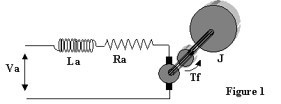
In Figure 1, the applied armature voltage is Va, the armature inductance is La and Ra is armature resistance. The inertia of the motor and load is J and the motor and load friction is represented by Tf.

This experiment (Parts I and II) will explore the characteristics of the DC servomotor and we will use the laboratory instrumentation to measure the parameters, which describe its behavior. This (Part I) focuses on the electrical parameters. Part II will address the mechanical characteristics of the motor and its dynamic behavior. The conclusion of this full experiment will have you using your measured characteristics of the motor to describe it mathematically and model it with MATLAB.

EQUIPMENT AND DATA COLLECTION

The first step in this sequence of parameter determination experiments is to measure the motor armature resistance. Unfortunately, the motor brushes have distracting contact characteristics, which make this process more complicated than using an ohmmeter. It takes a significant current to break down the contact resistance and establish the normal resistive behavior of the armature. Using your test motor and a shunt resistor, connect the circuit of Figure 2 with the power amplifier driving the system following the function generator input.

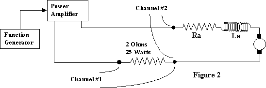
Set the function generator to a low frequency (approximately 0.2 Hz or less) and a triangular waveform with the offset adjusted to zero. The oscillating voltage across the shunt resistor (channel 1) should range over +/- 2 volts (+/- 1 amp). The motor will tend to rotate, clamp it with the torque calibration arm to prevent its motion. Capture a full cycle of the channel 1 and 2 voltage oscillations with the VB-Scope. Use Excel to convert the channel 1 signal to current and plot armature voltage vs. current. The slope of this plot is the armature resistance Ra. (This is required plot #1.)

The next test is to determine the armature inductance. Using the circuit arrangement of Figure 2, shift channel 2 to monitor the amplifier output voltage and change the waveform to a square wave (approximately 0.2 Hz or less). Again clamp the motor shaft. Observe the shunt resistor voltage of channel 1 - it should have an exponential form in response to the step changes in voltage input. And the steps in voltage input should be nicely "square". Use the VB-Scope to capture the channel 1 and 2 waveforms. (Set the VB-Scope Time-Base to 2 or 5 seconds or data rate to capture a sufficient number of points to get the detailed response - 5000 is suggested). Use Excel to obtain current from the channel 1 data and plot current vs. time. 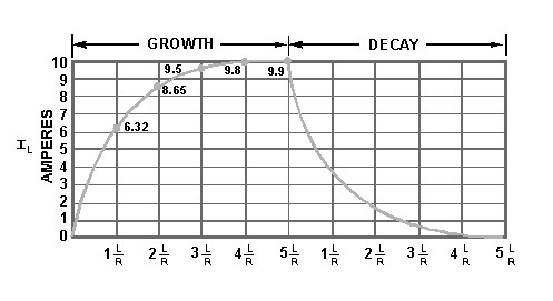(This is required plot #2.) The R-L circuit is a first order system with a time constant of L/R seconds. Recalling that the 2 ohm shunt resistance adds to the armature resistance in this arrangement, determine the armature inductance.

(Figure source: http://www.tpub.com/neets/book2/2d.htm)

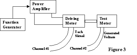
The final electrical test is to determine the motor back EMF coefficient Kg. The simple arrangement of Figure 3 below is used where a "driving motor" is employed to turn the "test motor". In this case, the motor tach voltage (channel 1) and the generated voltage from the test motor (channel 2) are monitored by the VB-Scope. The function generator is again set at a low frequency triangle wave with zero offsets. The amplitude should be adjusted so that the fluctuations in the motor speed tach signal and the generated test motor voltage do not exceed the range of the VB-Scope. Recall that the motor's built-in tach sensitivity is 16.5 volts/1000 rpm.

Use your VB-Scope to capture a full cycle of the waveforms for channels 1 and 2. Use Excel to generate a properly calibrated plot of generated voltage vs. motor speed in radians/sec. (This is required plot #3.) Determine the motor generator constant Kg from the slope of this plot. It should be in units of volts/rad/sec.

REPORT

There will be one report submitted for the complete Experiment 8. The report will be submitted in FULL report form after both parts of the experiment have been completed. Each individual must submit his own report in which written text should be prepared independent of your group partners. But you are welcome to work with your partners on data processing, graphs, the determination of system parameters and on a MATLAB simulation of the motor/load response to a step input.